Federgraph Formula
The formula of Sample 1
The Federgraph application does not only plot Betrag, Richtung, and Energie, but also something like abs(u), even if this is just for fun. Sample 1 in the Federgraph application uses the formula shown in the following image.
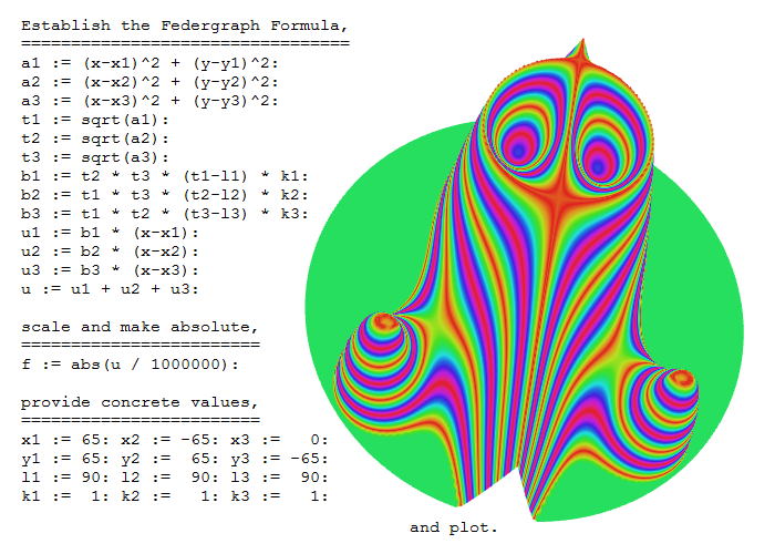
The formula above is given in Maple syntax.
Using an old version of Maple
The monument of Federgraph ancestors:
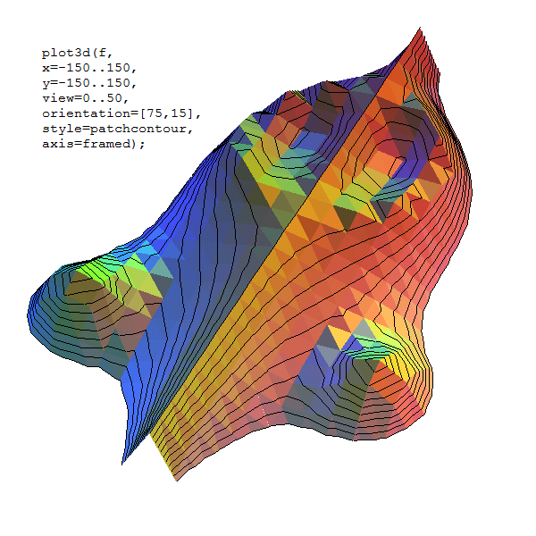
The image shows that the sample can be recreated in the old 16 bit student version of Maple, which I used back in 1994.
Using a current version of Maxima
Maxima is a free program you can use to prove it; just copy and paste the text out of the following preformatted paragraph into Maxima:
/* Establish the Federgraph formula */

a1: (x-x1)^2 + (y-y1)^2$
a2: (x-x2)^2 + (y-y2)^2$
a3: (x-x3)^2 + (y-y3)^2$

t1: sqrt(a1)$
t2: sqrt(a2)$
t3: sqrt(a3)$

b1: t2 * t3 * (t1-l1) * k1$
b2: t1 * t3 * (t2-l2) * k2$
b3: t1 * t2 * (t3-l3) * k3$

u1: b1 * (x-x1)$
u2: b2 * (x-x2)$
u3: b3 * (x-x3)$

u: u1 + u2 + u3$

/* scale and make absolute */

f: abs(u / 1000000)$

/* provide concrete values */

x1: 65$ x2:-65$ x3:  0$
y1: 65$ y2: 65$ y3:-65$
l1: 90$ l2: 90$ l3: 90$
k1:  1$ k2:  1$ k3:  1$

/* and plot */
plot3d(f, [x,-150,150], [y,-150,150],  [z,0,50],  [plot_format,gnuplot]);
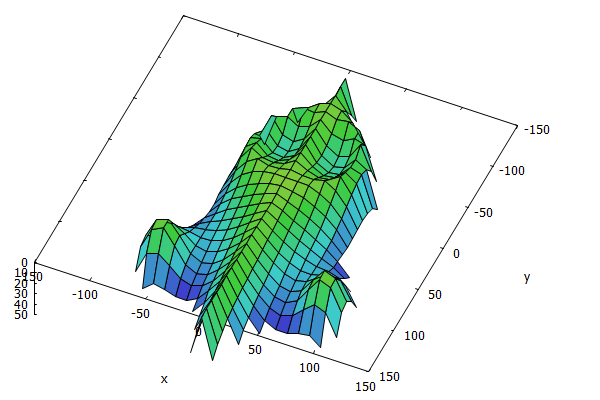
The image above is a screenshot of the gnuplot output.
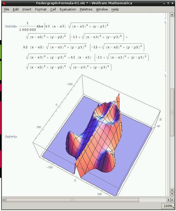
Using Mathematica
This will work on the Raspberry Pi where Mathematica is a free download.
(* Clear *)
ClearAll[x1, x2, x3]
ClearAll[y1, y2, y3]
ClearAll[l1, l2, l3]
ClearAll[k1, k2, k3]

(* Establish the Federgraph formula *)
a1=(x-x1)^2+(y-y1)^2;
a2=(x-x2)^2+(y-y2)^2;
a3=(x-x3)^2+(y-y3)^2;

t1=Sqrt[a1];
t2=Sqrt[a2];
t3=Sqrt[a3];

b1=t2*t3*(t1-l1)*k1;
b2=t1*t3*(t2-l2)*k2;
b3=t1*t2*(t3-l3)*k3;

u1=b1*(x-x1);
u2=b2*(x-x2);
u3=b3*(x-x3);

u=u1+u2+u3;

(*scale and make absolute*)
f= Abs[u/1000000]

(*provide concrete values*)
x1=65;
x2=-65;
x3=0;
y1=65;
y2=65;
y3=-65;
l1=90;
l2=90;
l3=90;
k1=1;
k2=1;
k3=1;

(*and plot*)
Plot3D[f,{x,-150,150},{y,-150,150}, PlotRange -> {0, 50}]
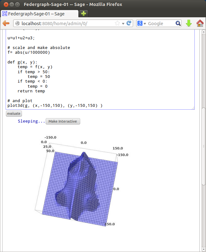
Using Sage
# provide concrete values
x1=65; x2=-65; x3=0
y1=65; y2= 65; y3=-65;
l1=90; l2= 90; l3= 90;
k1= 1; k2=  1; k3=  1;

# establish the Federgraph formula
x, y = var('x,y')

a1=(x-x1)^2+(y-y1)^2;
a2=(x-x2)^2+(y-y2)^2;
a3=(x-x3)^2+(y-y3)^2;

t1=sqrt(a1);
t2=sqrt(a2);
t3=sqrt(a3);

b1=t2*t3*(t1-l1)*k1;
b2=t1*t3*(t2-l2)*k2;
b3=t1*t2*(t3-l3)*k3;
u1=b1*(x-x1);
u2=b2*(x-x2);
u3=b3*(x-x3);

u=u1+u2+u3;

# scale and make absolute
f= abs(u/1000000)

def g(x, y):
    temp = f(x, y)
    if temp > 50:
        temp = 50
    if temp < 0:
        temp = 0
    return temp

# and plot
plot3d(g, (x,-150,150), (y,-150,150) )
Using HelixToolkit
u = (u - 0.5) * 300;
v = (v - 0.5) * 300;

double x1 = 65;
double x2 = -65;
double x3 = 0;

double y1 = -65;
double y2 = -65;
double y3 = 65;

double l1 = 90;
double l2 = 90;
double l3 = 90;

double k1 = 1;
double k2 = 1;
double k3 = 1;

double a1, a2, a3;
double b1, b2, b3;
double t1, t2, t3;
double u1, u2, u3;

x = u;
y = v;

a1 = (x - x1) * (x - x1) + (y - y1) * (y - y1);
a2 = (x - x2) * (x - x2) + (y - y2) * (y - y2);
a3 = (x - x3) * (x - x3) + (y - y3) * (y - y3);

t1 = Math.Sqrt(a1);
t2 = Math.Sqrt(a2);
t3 = Math.Sqrt(a3);

b1 = t2 * t3 * (t1 - l1) * k1;
b2 = t1 * t3 * (t2 - l2) * k2;
b3 = t1 * t2 * (t3 - l3) * k3;
u1 = b1 * (x - x1);
u2 = b2 * (x - x2);
u3 = b3 * (x - x3);

z = u1 + u2 + u3;
z = Math.Abs(z / 1000000);

if (z > 50)
    z = 50;
if (z < 0)
    z = 0;

z = -z;
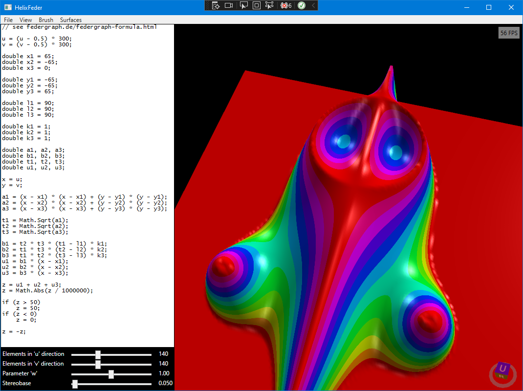
21st century X-Eyes
If you change the texture parameters, Federgraph kind of rolls its eyes. It may be regarded as a modern age (GPU intensive) alternative to X-Eyes, which you must see live!